
Mathematical Modeling of FDG Concentration in Brain Tissue
Fall 2024 · Mathematical Methods · Johns Hopkins University
Project
This project solves the system of coupled ordinary differential equations governing the rate of change of FDG (fluorodeoxyglucose) in brain tissue. The analysis uses Laplace transforms to derive an analytical solution expressed as convolution integrals, then applies numerical integration (MATLAB's ode45) to compute concentration over time from tabulated blood-plasma data. The results inform optimal PET scan timing for maximum image contrast.
1. Analytical Solution via Laplace Transforms
Solve the system of coupled differential equations that govern the rate of change of FDG in brain tissue. Using Laplace transforms, express the equations as convolutions and reproduce the target formula:
Governing Equations
Equation (1) — Free FDG in brain tissue:
$$\frac{dC_e}{dt} = k_1 C_p - (k_2 + k_3)C_e + k_4 C_m$$- $k_1 C_p$: rate of transport of FDG from blood plasma into the brain
- $-(k_2 + k_3)C_e$: rate of loss from the free compartment ($k_2$ = return to blood, $k_3$ = phosphorylation/trapping)
- $k_4 C_m$: trapped FDG-6-P reverting back into free FDG
Equation (2) — Trapped FDG-6-P:
$$\frac{dC_m}{dt} = k_3 C_e - k_4 C_m$$- $k_3 C_e$: rate of conversion of free FDG to trapped FDG-6-P
- $-k_4 C_m$: return of FDG-6-P back into free FDG
Initial conditions: At $t = 0$, $C_e(0) = 0$, $C_m(0) = 0$.
Laplace Transform Derivation
The Laplace transform of a function $f(t)$ is:
$$\mathcal{L}\{f(t)\} = F(s) = \int_0^\infty f(t)\,e^{-st}\,dt$$Applying the Laplace transform to both governing equations with zero initial conditions:
Equation 1 in $s$-space:
$$(s + k_2 + k_3)\,C_e(s) = k_1\,C_p(s) + k_4\,C_m(s)$$Equation 2 in $s$-space:
$$(s + k_4)\,C_m(s) = k_3\,C_e(s) \quad\Longrightarrow\quad C_m(s) = \frac{k_3\,C_e(s)}{s + k_4}$$Substitution and Simplification
Substituting $C_m(s)$ into Equation 1 and solving for $C_e(s)$:
$$C_e(s) = \frac{k_1\,C_p(s)(s + k_4)}{s^2 + (k_2 + k_3 + k_4)s + k_4 k_2}$$Back-substituting to get $C_m(s)$:
$$C_m(s) = \frac{k_1 k_3\,C_p(s)}{s^2 + (k_2 + k_3 + k_4)s + k_4 k_2}$$The total brain tissue concentration $C_i(s) = C_e(s) + C_m(s)$:
$$C_i(s) = C_p(s) \cdot \frac{k_1(s + k_4 + k_3)}{s^2 + (k_2 + k_3 + k_4)s + k_4 k_2}$$Factoring the Denominator
Let $\alpha_1, \alpha_2$ be the roots of the quadratic denominator, found via:
$$\alpha_{1,2} = \frac{-(k_2 + k_3 + k_4) \pm \sqrt{(k_2 + k_3 + k_4)^2 - 4k_4 k_2}}{2}$$Then perform partial fraction decomposition:
$$C_i(s) = C_p(s) \cdot \left(\frac{A}{s - \alpha_1} + \frac{B}{s - \alpha_2}\right)$$Matching coefficients from $k_1(s + k_4 + k_3) = A(s - \alpha_2) + B(s - \alpha_1)$:
Inverse Laplace Transform & Convolution
Using the convolution property of the inverse Laplace transform, the final solution in the time domain is:
This reproduces the target formula (4) from the associated paper.
2. Numerical Integration & Optimal Scan Timing
Using tabulated concentration data of FDG in blood, numerically compute the concentration in brain tissue $C_i(t)$ over time via MATLAB's ode45 solver.
Rate Constants
| Parameter | Value |
|---|---|
| $k_1$ | 0.102 |
| $k_2$ | 0.130 |
| $k_3$ | 0.062 |
| $k_4$ | 0.0068 |
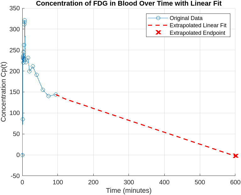
Blood Concentration Data & Extrapolation
The provided blood-plasma concentration data was extended with a linear fit to estimate the time at which FDG concentration reaches zero (~600 min).
ODE System & MATLAB Implementation
The coupled ODEs were solved numerically using ode45 with interpolated blood-plasma data as the driving input. The ODE system:
MATLAB code for the numerical solution:
% Rate constants
k1 = 0.102; k2 = 0.130; k3 = 0.062; k4 = 0.0068;

% Original data
time_data_original = [0, 1.08, 1.78, 2.30, 2.75, 3.30, 3.82, 4.32, ...
    4.80, 5.28, 5.95, 6.32, 6.98, 9.83, 16.30, 20.25, ...
    29.67, 39.93, 58.00, 74.00, 94.00];
Cp_data_original = [0, 84.9, 230.0, 233.0, 220.0, 236.4, 245.1, ...
    230.0, 227.8, 261.9, 311.7, 321.0, 316.6, 220.7, ...
    231.7, 199.4, 211.1, 190.8, 155.2, 140.1, 144.2];

% Extended data with linear decay to zero
time_data_extended = [time_data_original, 120, 180, 240, 300, 400, 500, 600];
Cp_data_extended = [Cp_data_original, 100, 50, 30, 10, 5, 2, 0];
Cp_interp = @(t) interp1(time_data_extended, Cp_data_extended, t, 'linear', 'extrap');

% ODE system
function dydt = odesystem(t, y, k1, k2, k3, k4, Cp_interp)
    Ce = y(1); Cm = y(2);
    Cp_t = Cp_interp(t);
    dCe_dt = k1 * Cp_t - (k2 + k3) * Ce + k4 * Cm;
    dCm_dt = k3 * Ce - k4 * Cm;
    dydt = [dCe_dt; dCm_dt];
end

initial_conditions = [0, 0];
[t_out, y_out] = ode45(@(t,y) odesystem(t, y, k1, k2, k3, k4, Cp_interp), ...
    [0 600], initial_conditions);

Ci_t = y_out(:,1) + y_out(:,2);
Results
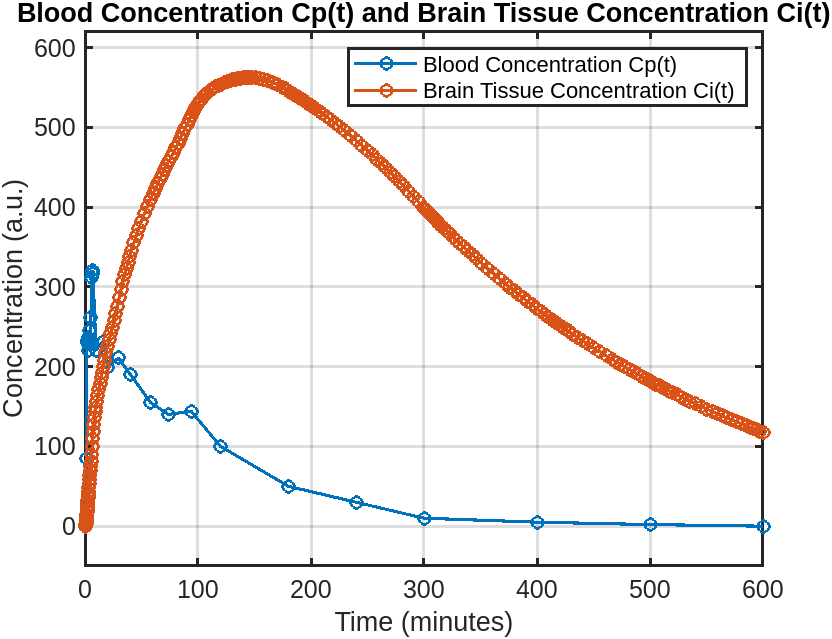
Peak Concentration: $C_i = 562.71$ (a.u.)
Time to Peak: $t = 144.5$ minutes
Interpretation & Optimal Scan Window
After injection of isotope-tagged FDG, the brain concentration $C_i(t)$ gradually increases, reaching a peak at approximately 144.5 minutes. After this peak, the concentration declines as the body metabolizes and clears FDG from the brain.
Scanning between 100 and 200 minutes post-injection — centered around the time to maximum concentration — would yield the highest isotope-tagged FDG concentration in brain tissue, producing higher contrast in PET images and ensuring optimal image quality.
Appendix: Computed Concentration Data
Full numerical output of $C_i(t)$ computed via ode45 (245 data points). A subset is shown below:
| Time (min) | $C_i$ (a.u.) |
|---|---|
| 0.000 | 0.000 |
| 0.199 | 0.158 |
| 0.599 | 1.399 |
| 0.998 | 3.760 |
| 1.770 | 14.698 |
| 3.000 | 39.231 |
| 5.041 | 74.661 |
| 6.998 | 109.377 |
| 9.469 | 148.757 |
| 13.316 | 178.763 |
| 16.945 | 207.367 |
| 22.851 | 241.357 |
| 28.534 | 275.820 |
| 35.258 | 316.051 |
| 41.072 | 345.146 |
| 49.859 | 382.166 |
| 57.799 | 409.396 |
| 68.382 | 441.426 |
| 76.317 | 463.244 |
| 84.309 | 486.335 |
| 92.302 | 509.848 |
| 99.466 | 528.445 |
| 106.631 | 541.035 |
| 115.221 | 550.769 |
| 126.221 | 557.406 |
| 135.366 | 561.217 |
| 144.510 | 562.713 |
| 157.564 | 560.584 |
| 174.803 | 550.390 |
| 192.488 | 534.488 |
| 213.410 | 514.107 |
| 250.305 | 470.740 |
| 299.686 | 399.797 |
| 350.762 | 329.985 |
| 399.612 | 273.265 |
| 444.573 | 228.595 |
| 496.141 | 185.058 |
| 545.324 | 150.117 |
| 600.000 | 117.638 |